Machine Learning in Finance: An innovative approach to analysing Hidden Reserves / Losses processes and other financial parameters

Photo by Marcus Lenk on Unsplash on 15.01.2021

In this article, the use of scripting and innovative machine learning techniques to automate and improve on the analysis of the Hidden Reserves and Losses (HRL) processes, which is commonly performed in the Finance departments of banks, is described. It is demonstrated how numerous quantitative effects, which define the components of the change in the HRL, can be categorised, explained, and illustrated using various machine learning algorithms.

The HRL process is considered solely to demonstrate the techniques by using an underlying example. The approach outlined in this article is not restricted to this example but is universally applicable whenever a financial parameter, whose value is influenced by various underlying features, e.g., spreads, interest curves, etc., must be analysed to determine the driving factors of its change from one point in time to another.

Introduction to the HRL process

Hidden reserves and losses describe unrecognised positive and negative valuation effects of at cost accounted financial instruments that arise from the difference in book value and market value.

Based on this classification, the HRL for a single financial instrument is defined according to the following formula:

Equation 1: Definition of HRL

where the market value (MV) is the fair value of an instrument and the book value (BV) is the carrying value of the instrument on the balance sheet.

The change in HRL (∆HRL) is usually calculated over a certain period, e.g., three months, and is defined as follows:

Equation 2: Definition of ∆HRL

Here, ∆MV and ∆BV are given by

Equation 3: Definition of ∆MV

and

Equation 4: Definition of ∆BV

respectively, with dates t₂ > t₁.

Repeatedly calculating ∆HRL for a big portfolio is rather labour-, time- and resource-intensive and generally involves manual copying, moving, pasting of data and subsequently the analysis of the changed market and book values and its outliers.

This leads to various possibilities of how to further digitalise and optimize the process of calculating the ∆HRL for portfolios, namely finding sophisticated approaches of how to

Automate data processing,
Perform feature engineering and selection,
Explain the change in the HRL.

In the ML approaches described in this article, the data required includes market values and book values, as well as their components, i.e., features, in addition to yield curves, spreads and exchange rates.

AUTOMATED DATA PROCESSING WITH RPA AND/OR PYTHON

To calculate the HRL of an instrument and particularly to analyse the reasons for changes in the HRL from one date to another, it is usually required to extract data from various systems. In this context, it is important to remember that market and book values are not just single variables but are defined themselves by various parameters (or features). For example, the book value of an instrument consists of parameters such as the notional, premium discount fees, other fee types, amortisation costs, etc. Equally, the market value of an instrument is defined by features such as the interest curve, spreads, etc.

Manual processing of the different data sources generally requires the manipulation of complex data structures in Excel sheets, which is resource-intensive and prone to inadvertent errors.

A better approach to manipulate the underlying data in a manner which makes it accessible for the machine learning algorithms described in this article, is to automate the data processing using digital resources such as Robot Process Automation (RPA) or the scripting language Python, which has built-in libraries for data manipulation. This provides more transparency, makes it easier to track changes, simplifies the identification of errors in the data processing steps that are rule-based and immune to human error and, in addition, provides significant time-savings.

The detailed description of such data manipulations is not in the scope of this article.

FEATURE ENGINEERING, SELECTION AND HRL EXPLANATION USING MACHINE LEARNING

Having built the basic requirements for transforming the raw input data into a format that can be processed by the machine learning algorithms, one can proceed to build a model that explains the changes in the HRL from one date to another based on its selected or predefined features.

In this context, the first step involves determining which features should be used in the model. One approach is to consider the theoretical relationships between the target variable (HRL) and variables that can potentially explain its change. For example, since ΔHRL can be written as the difference between the change in market value and the change in book value (see Equation 2), it makes sense to analyse the features that influence the components ΔMV or ΔBV, respectively.

In the following, the focus is on finding features that explain ΔMV, however, the techniques described may be applied in an equal measure to ΔBV.

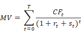
The general formula used to calculate the market value of a financial instrument, e.g., a bond, is given by:

Equation 5: Definition of MV

In this formula, the future cashflows (CF_t) at different points in time t are discounted using risk-free interest rates (r_t) and spread values (s_t).

Example

From Equation 5, it follows that an inverse relationship between interest rates, spreads and the market value exists. Higher interest rates or spread values lead to higher discount rates and thus to lower market values. If the book value does not change or rises simultaneously, the relationship in Equation 1 implies a lower HRL.

The example outlines that interest rates and spreads may define two feature variables for explaining differences in HRL.

Having determined a sufficiently large set of feature variables that can potentially be used to explain the ΔHRL, the next step is to select a subset, i.e., only those that provide the most meaningful explanation for the HRL movement.

One ML (analysis) method that can be used for variable (feature) selection in the context of regularisation is the so-called lasso (least absolute shrinkage and selection operator). It is widely used to reduce the set of known covariates (in our case the initial features) and to enhance the interpretability of the resulting statistical model. Mathematically, the goal is to find the vector β_lasso that minimizes the lasso loss function[1] ℒ:

Equation 6: Definition of β_lasso

It can be observed that the objective function on the right-hand side of the expression in Equation 6 represents a trade-off between the goodness of fit and the absolute value of the coefficients, controlled by the regularization hyperparameter λ. High values of λ lead to a lower sum of the absolute values of the optimal coefficients in ‖β‖₁ and low values bring the coefficients closer to the ones estimated by a linear regression using an ordinary least squares (OLS) method. The optimal value of λ is chosen by cross-validation[2].

It can be shown that lasso estimator tends to yield solution vectors β_lasso where some of the entries are zero. Since the entries of β_lasso can be interpreted as importance weights of the features, this is a useful property that is used to select the most meaningful features from the initial set of p candidates.

As already described, the optimal value of the regularization hyperparameter is selected by cross-validation and the resulting lasso regression is subsequently applied to the data set. The estimate of β_lasso is sparse, meaning that some of its values are close to or exactly equal to zero. The corresponding features are regarded as not meaningful and are not used in the later stages of the analysis. Other features, whose respective coefficients are far away from zero, are considered as important.

Having selected the meaningful features via lasso regression, the goal is to estimate their effect on the target variable, namely ΔHRL. This can be achieved by a linear regression model, which tries to estimate the coefficients β_i in the following functional relationship:

Equation 7: Linear regression model

In Equation 7, y_j is the value of the target variable (ΔHRL in our case) for observation (financial instrument) j, elements of {x_ij}^p_i=1 are values of features (for instance, a change in the interest rate) for observation j and {β_i}^p_i=1 are coefficients, i.e., parameters of the model which need to be estimated.

The coefficients can be estimated by solving an ordinary least squares (OLS) optimization problem[3]:

Equation 8: Ordinary least squares optimization problem

The OLS optimization problem presented above focuses, for mathematical reasons, on minimizing the squared residuals of the linear regression rather than the mean absolute values directly.

As a result, the residuals with a high absolute value influence the solution more strongly and make the model less generalizable. To mitigate this effect, one can eliminate the outliers in the distribution of the target variable by setting its values below the α quantile to the α quantile value and values above the (1 - α) quantile to the (1 - α) quantile value. α in the example above is typically small, i.e., 0.01 or 0.025.

Having estimated the coefficients using the OLS approach, one can easily estimate effects of single features on the target variable for groups of instruments or even a particular financial instrument. This is achieved by multiplying values of the features for the instrument with the respective coefficients.

PRACTICAL IMPLEMENTATION

The theoretical approach outlined in the previous section, which can be used to explain the determining features that drive ΔHRL, or, more particularly ΔMV, has opened the path for a practical implementation.

In the previous sections, it was argued that based on theoretical considerations it is, e.g., reasonable to include changes in interest rates and spreads as features. Along with these two variables, continuous features[4] such as book value (ΔBV), notional (ΔN) and fair value adjustment (ΔFVA) changes, as well as categorical features[5] such as hedging and currency information may also be favourable for explaining the changes in ΔHRL and can therefore be incorporated into the analysis.

The application of the lasso regression estimator to the underlying dataset can theoretically lead to the elimination of either continuous or categorical features. For the portfolio that forms the basis of this analysis, the coefficients of the categorical features are set to zero, which basically means that they are not meaningful in the further analysis. This is due to the properties of the lasso model and the data at hand.

The remaining (continuous) features define the respective parameters (y_j, {x_ij}^p_i=1 and {β_i}^p_i=1) of the ordinary linear model stated in Equation 7 and thus form the functional relationship between ΔHRL and the explanatory variables/features (see Equation 9). Using the data for the entire portfolio and by solving the OLS optimization problem presented in Equation 8, the estimates of the parameters {β_i}^p_i=1 can be calculated, which are displayed as numbers in Equation 9 below. These parameters capture the functional relationship between the target variable ΔHRL (y_j in Equation 7) and features, such as ΔIR, ΔBV and others ({x_ij}^p_i=1 in Equation 7).

Equation 9: Functional relationship between ∆HRL and selected features

In terms of the coefficients signs, Equation 9 shows that the model captures negative relations between the ΔHRL and changes in spreads (ΔS) and interest rates (ΔIR).

Using the estimated linear function, it is now possible to calculate the approximate effects of the features on the target variable for a single financial instrument. To do so, one must multiply the estimated coefficients with the values of the explanatory variables. In terms of Equation 7, one such effect for feature i can be presented as a product β_i x_ij, where β_i is the i-th coefficient and x_ij is the i-th explanatory variable/feature for the j-th financial instrument. Using the estimates in Equation 9, the effect of the interest change on ΔHRL can be calculated by multiplying the value of the respective coefficient (-374,147) with the value of the feature (ΔIR).

Values in EUR	ΔMV	ΔBV	ΔHRL
Loan 1	809,565	1,253,115	-443,550
Loan 2	-184,365	-322,602	138,013

Table 1: Breakdown of ΔHRL in EUR for two specific examples of distinct loans into ΔMV and ΔBV.

In Table 1, ΔHRL calculations based on changes in book and market values are presented for two individual loans. It can be observed that Loan 1 experiences a ΔHRL reduction, because the growth of ΔBV outweighs the increase of ΔMV. On the other hand, Loan 2 shows an increase in ΔHRL since the decrease of ΔBV is greater than the decline of ΔMV.

Based on the linear model shown in Equation 9 and the two loans stated in Table 1, the effects of single features on ΔHRL can now be estimated[6]. They are presented in Figure 1 and Figure 2.

Figure 1: Breakdown of ΔHRL in EUR for Loan 1 into various effects. The positive effects are displayed as green bars, negative effects as red bars and the prediction of the HRL change is visualized as a blue bar. As reference, the real HRL change (ΔHRL) is displayed as a grey bar.

As stated above, the effect of a single feature is determined, by multiplying the coefficient of the linear model with the corresponding value of the explanatory variable. For example, if the book value change for loan 1 equals 1,253,115 EUR and the coefficient equals -0.38, then the effect of ΔBV can be calculated as

Equation 10: Approximative calculation of the effect of ∆BV on ∆HRL

It should be noted that the approach presented in this article does not generate a perfect estimate when calculating the effects on an instrument level. This leads to differences between the ΔHRL estimated using the model presented and the actual ΔHRL. These errors cancel out on a portfolio level due to certain mathematical properties of the problem. Despite the imperfect precision, which can be improved by adding more features and/or by applying more sophisticated machine learning models, the big advantage of the linear regression approach is its interpretability, which makes the calculation of the abovementioned effects possible.

The calculation of the effects for the other variables/features can be performed in the same manner.

Figure 2: Breakdown of ΔHRL in EUR for Loan 2 into various effects. The positive effects are displayed as green bars, negative effects as red bars and the prediction of the HRL change is visualized as a blue bar. As reference, the real HRL change (ΔHRL) is displayed as a grey bar.

The (visual) representation allows to determine which effects have had the strongest influence on ΔHRL. For instance, for the first loan the change in book value is the most significant parameter (see Figure 1). In case of the second loan, the change in interest rates has the most profound effect on the target variable (see Figure 2).

Conclusion

Machine learning technology has had a profound effect on various business areas and on the financial services industry in general. The application of specific algorithms and labelled data has enabled professionals to improve on the approximation and the prediction of quantitative effects, to explain underlying effects and to increase the performance of such calculations considerably.

Together with automated rule-based pre-processing, the new techniques can give financial professionals a significant advantage when processing and identifying irregularities (or exceptions) that may be hiding in their data.

The machine learning based technique outlined in this article supports these claims and clears the path for a quick and coherent explanation of underlying effects when investigating parameters such as the fair value or book value of financial instruments. In this context, the application of the technique is not restricted to the HRL process, which is solely used as an example in this article but can be applied in all areas where the value of such parameters is determined by various underlying figures.

OUR OFFER

The ML algorithms and methodical rule-based automation approaches presented in this document allow for various possible implementation strategies for financial institutions, e.g., in processes such as the determination of HRL, hedge accounting, etc.

We would be pleased to advise you on different possible ML applications combined with automation and to help you to develop the solution which, within the professional and technical possibilities, is adequately suited for your company.

References

[1] In the expression y is a n-dimensional (n ≙ #observations) target vector that contains the target values (in our case the ΔHRL for single financial instruments). X is a n × (p + 1) matrix of features arranged column-wise, e.g., spreads or interest rate changes, where (p + 1) is the number of those features (in our case p features in the initial set) plus the constant term. β and β_lasso are also (p + 1)-dimensional vectors, their dimensionalities are equal to the number of columns in the matrix X. λ ≥ 0 is a scalar regularization hyperparameter that indicates the degree to which high components of β are penalised (the case λ = 0 gives back the ordinary least squares OLS method). The associated norms are ℓ₁ and ℓ₂.

[2] During the cross-validation process, the estimator is repeatedly applied to one part of the dataset and evaluated on another one for various values of the regularization hyperparameter. Eventually, the parameter value that achieves an optimal out-of-sample performance on the holdout data, is selected.

[3] The OLS optimization problem is a special case (for λ = 0) of the lasso optimization problem. The characteristics (variable definitions, dimensions, etc.) are the same as in the lasso regression optimization problem – these can be found in footnote 1.

[4] Continuous features can achieve a real number value with arbitrary precision. For example, the book value of a financial instrument can be theoretically equal to any non-negative number.

[5] Categorical features can only be equal to a limited number of values. For instance, the currency feature in any given dataset may only have the following values “EUR”, “USD”, “CHF” and “GBP”.

[6] The features ΔFVA, ΔIR, ΔN and ΔS are not explicitly stated in Table 1.